Three Discrete Sampling Methods
This post describes and implements three methods which can be used to sample from any discrete probability distribution.
Probability integral transform
The first method is an “implementation” of the probability integral transform theorem. The theorem states that, for any continuous random variable \(X\) with cumulative distribution function (CDF) \(F_X\), \(Y = F_X(X)\) has uniform distribution. We can invert the equation above to sample from any continuous distribution. More concretely, we first sample \(y \sim U\) then use the inverse CDF to get \(x = F_X^{-1}(y)\) where \(x \sim X\). Although the probability integral transform is defined for continuous random variables, it can be shown to hold for discrete variables as well.
Unlike continuous variables, obtaining the CDF for discrete variables is trivial. The CDF is equal to the cumulative sum of the probability mass function (PMF). Given discrete random variable \(X\) with PMF \([p_0, p_1, \dots, p_N]\), its CDF \(F_X\) is simply \([p_0, p_0 + p_1, \dots, p_0 + p_1 + \dots + p_N]\).
Putting everything together, to sample from any discrete probability distribution, we first sample \(y \sim U\) then return the last state where \(F_X < y\). Here’s what that looks like in Python:
from typing import List
import numpy as np

def sample(cdf: List[float]) -> int:
    y = np.random.uniform()
    idx = 0
    while cdf[idx] < y:
        idx += 1
    return idx
We can see by inspection that each sample takes \(O(N)\) time, where \(N\) is the number of states \(X\) can take. Can we do better?
Binary search
One straightforward extension is to realize that the CDF is monotonic and hence sorted. We can use binary search to drive the runtime complexity to \(O(\log N)\). In Python this can be implemented in two short lines of code:
from bisect import bisect

def sample_binary_search(cdf: List[float]) -> int:
    u = np.random.uniform()
    return bisect(cdf, u)
Can we do even better?
Walker’s Alias Method
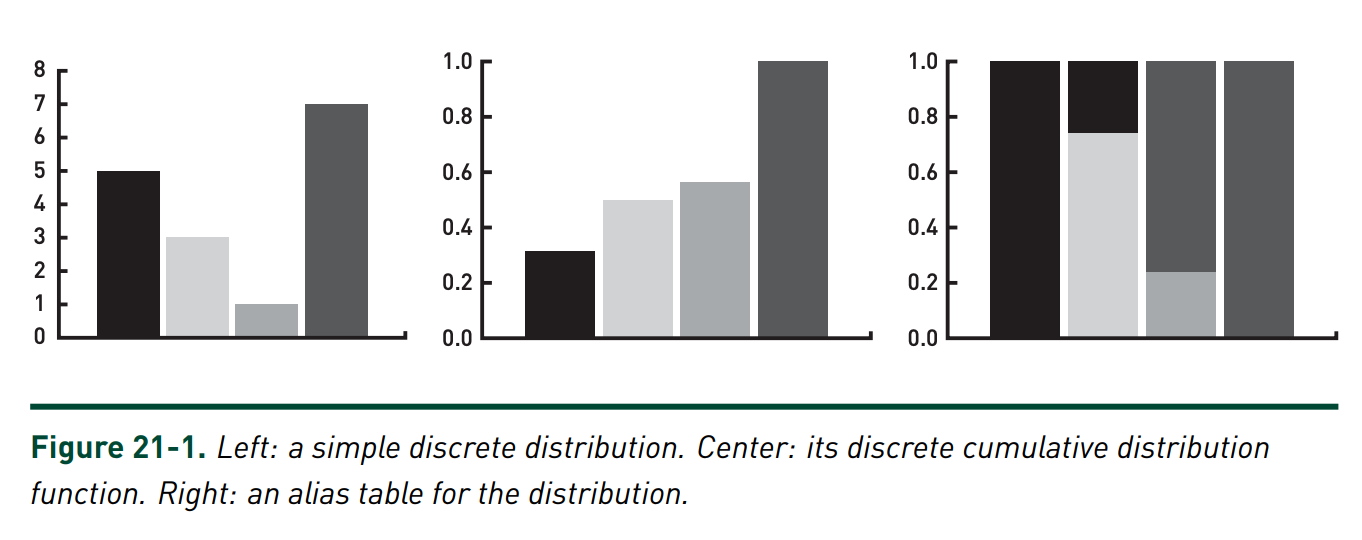
The optimal sampling method, know as Walker’s alias method, can sample from any discrete distribution in \(O(1)\) time. The basic intuition behind the method is to transform the PMF of a random into a 2d rectangle (as shown in Figure 1), randomly sample \(x, y\) coordinates inside the rectangle, and return the corresponding state aliased to those coordinates.
 |
Although the intuition is straightforward, creating the alias table (Figure 1 right) and using it for sampling is somewhat involved. I found [1] gave a very clear description of how to do this, which I’ve implemented in Python below.
import copy

def construct_table(pmf: List[float]) -> List[Tuple[float, int, int]]:
    pmf, mean, table = copy.copy(pmf), np.mean(pmf), []
    for i in range(len(pmf)):
        idxs = np.argsort(pmf)
        i, j = idxs[i], idxs[-1]
        tau = pmf[i] / mean
        table.append((tau, i, j))
        pmf[j] -= mean - pmf[i]
        pmf[i] = 0  # Set to 0 to maintain correct sorting.
    return table

def sample_alias(alias_table: List[Tuple[float, int, int]]) -> int:
    N = len(alias_table)
    u_1, u_2 = np.random.uniform(), np.random.uniform()
    tau, i, j = alias_table[int(u_1 * N)]
    return i if u_2 < tau else j
Assuming we precompute the alias table, it’s evident that the runtime complexity is indeed \(O(1)\) for each sample.